Full Deployment Demo
This demo illustrates how to use and integrate exa4mind components using data created as part of a PhD thesis project. The source code for the demo can be found on IT4I's opencode Gitlab.
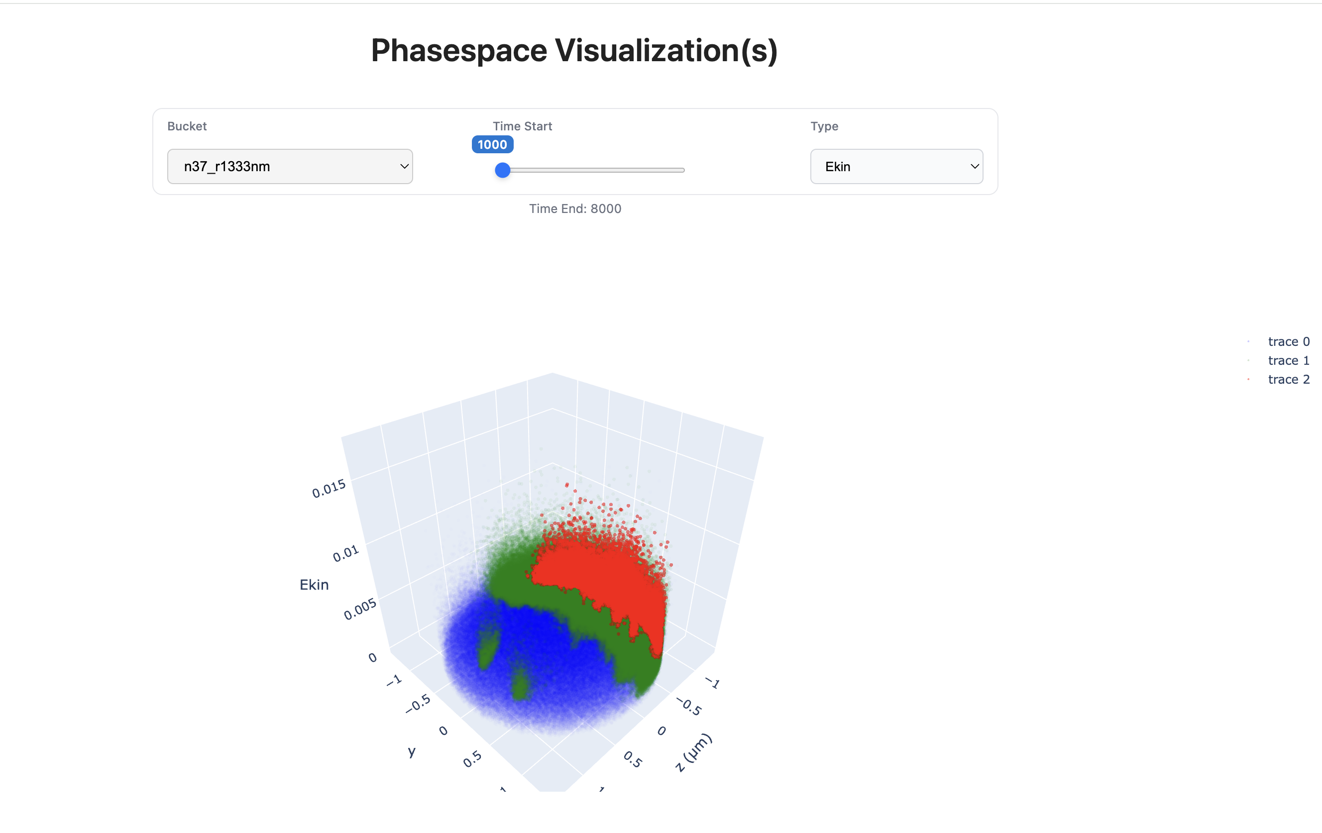
The goal of this demo is to visualise the effects of a very strong, very short laser pulse pulses being shot at a micrometer sized ion ball of gas or plastic. As they interact, the electromagnetic fields are so powerful that electrons are pulled out of the atom cores, leading to a charge surplus. This makes the ion ball explode, and the ions gain a lot of kinetic energy. Fast particles have many uses in the medical field and for kick-starting controlled fusion reactions, which are normally created using huge magnetic coils. The benefit of a laser based approach is a much smaller set-up. The data of how particles interact is the result of very large simulations, where the results include the position of electrons and protons in a 3D space. We visualise the position (y and z position in 3d space) and either the momentum (pz) or kinetic energy (Ekin) of the protons over time. This allows for insight in how changing parameters of the experiment affect the plasma creation.
The demo provides interactive visualisations rather than static PNGs, and is designed to make iteration straightforward. It is organised into three stages, allowing users to modify the data source or the visualisation code and create or regenerate visualisations by rerunning a one or two Airflow workflow(s).
Prerequisites
This demo is intended to run on a standard Linux system.
The following components are required:
- FAIR data subsetting API
- AQIS Engine with Airflow
- Dask
- A Flask-based webserver for serving the generated visualisations
The required packages are listed in pyproject.toml.
Both Airflow and the Flask webserver are expected to run on the same machine.
The Flask application reads visualisation files directly from the Airflow output directory via the local filesystem, in a folder named airflow_output.
This folder is located at the root directory from which the Airflow server was started.
FAIR Data
The first stage is using the FAIR data subsetting API to create the data product, i.e. the data to visualise. To create the product, a UUID to query mapping needs to be created.
In the demo, we use hdf5 files, where each file contains the data of one timestep for one simulation run This data is stored on the LRZ datastorage systems, and is accessible over an S3 compatible API. To make this data available outside of these systems, we use the FAIR data subsetting API to create a UUID for each hdf5 file. With the help of airflow, this process is automated.
Using the workflow
Using the create_mappings_airflow DAG in airflow/dags/create_mappings.py, you just need to give a bucket name where the data is stored.
In addition, a step value can be set, which controls in what increments the UUIDs for the files are created, e.g. for step=100, a UUID would be created for step 0, 100, 200, ...
There is also a check_s3_path option, which can check whether the files exist inside the buckets at the correct path.
For it to work, the s3proxy_conn_id variable in airflow needs to have valid credentials to the S3 store (see instructions here).
The information about which UUID corresponds to which timestep and simulation run is saved by airflow into the airflow_output/mappings.json file, e.g.
{
    "8d0280de-3c16-481c-a3d8-b5407d21b673": {
        "data_folder": "n192_r1333nm",
        "file_name": "pagg-t004000.h5"
    }
}
We can check the airflow logs to see that the mappings for the various files have been generated.
Please see ID-to-Dataset Resolution for a more thorough explanation and walkthrough of the UUID creation process.
Generating the Visualizations
In the second stage, we use the AQIS Engine with Airflow and Dask to create the interactive visualizations.
The workflow file can be found in the repo under airflow/dags/create_phasespace_aqis.py.
Import this into an existing Airflow system or create a new one.
Using the workflow
To run the workflow, select the create_phasespace_figures_dask DAG and click the "Trigger DAG" button.
Airflow will ask for the bucket/folder of the data we want to visualise, which needs to be one that was created in the first step.
Enter it and click run.
The data is retrieved from the FAIR data subsetting API with the UUIDs stored in airflow_output/mappings.json (created in the previous step).
We use Plotly to generate each visualisation as an HTML snippet.
The data is generated for the timesteps defined in the DAG, e.g. t=1000 to t=8000.
The system uses Dask to run the download and generation steps in parallel.
To create further visualisations, re-run the DAG with a different bucket name.
You can also change which timesteps should be generated inside the DAG code (t_firsts).
Info
Plotly uses a lot of RAM for generation. To prevent system slowdowns, the amount of parallel workers can be changed by adding the following in the dag file:
my_connection["dask_default"].extra["n_workers"] = <number of workers> # default: 4
All results, including the HTML snippet, are saved in the airflow_output folder.
The folder structure is flat, and each visualisation file name its type (ekin/pz), bucket name and the timestep.
Information about which visualisations have been created and when (timestamp) is saved by Airflow in airflow_output/phasespace.json.
The format of the JSON is defined in src/Fasttracker_phasespace_util.py as JSONFigureGroup.
The code to generate the visualisation are stored as separate files under the src/ folder in the repo and the relevant functions are imported.
This allows for changes to be made to the visualisation code without needing to touch the Airflow code.
Interacting with the Visualisations
In the third stage, we now want to interact with the visualisations, which look as follows:
Webserver
A Flask webserver serves the webpage, which includes the Plotly snippet from stage two.
The server reads snippets from the shared airflow_output directory.
The server does not need to be restarted when new visualisations are generated, the webpage just needs to be reloaded.
To start the webserver, run
flask --app main run --debug
from the same directory where the Airflow server was started. You can then navigate to the URL that is printed. The default is http://127.0.0.1:5000.
Using the GUI
The top of the page has 3 selectors to select the bucket, the timestep and the type of visualization (Ekin/pz).
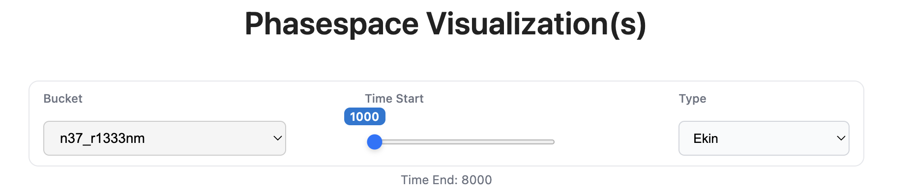 To change which figure to show, either select a different bucket or type or move the timestep slider.
It might take some time to load, as larger Plotly figures use a lot of system resources.
Warning
Loaded figures are not removed from memory, so selecting many will use large amounts of RAM. Close and reopen the webpage if the memory usage starts to become high.
You are able to interact with a plot directly by moving, zooming and rotating. You are also able to download a PNG of the current view with the "camera" button:
